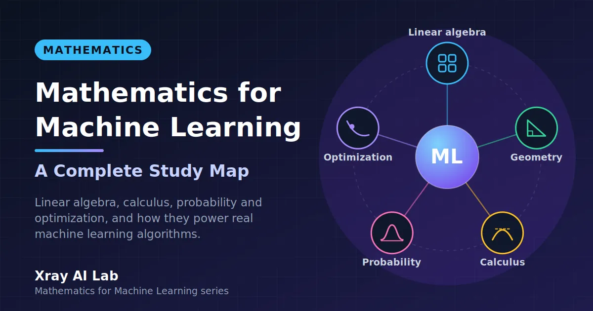
Mathematics for Machine Learning: A Complete Study Map

You can train your first machine learning model in a few lines of code. Import a library, call fit(), call predict(), and numbers come out. That is a great way to start, and nobody should wait to master mathematics before trying it. But sooner or later, a model behaves strangely. The loss stops decreasing, two features turn out to be nearly identical, or a result looks confident and is wrong. At that point, the difference between using a library and understanding it becomes very practical.

Mathematics is the language machine learning is written in. Data becomes vectors and matrices. Learning becomes the search for parameters that make a measurable error small. Uncertainty is handled with probability. Understanding that language does not mean proving theorems. It means being able to read what an algorithm is actually doing and to reason about why it works, why it fails, and what to change.

This article is the entry point to a series called Mathematics for Machine Learning. It gives you a map: which areas of mathematics matter, how they connect, in what order you can study them, and what you can safely postpone. It is deliberately a map, not a textbook. The detailed explanations come in the linked follow-up articles.

A note on sources. The structure below is my own suggested learning sequence. It is inspired by the general subject matter of the book Mathematics for Machine Learning by Deisenroth, Faisal, and Ong (Cambridge University Press, 2020), which is a good companion text, but it is not a summary of that book or of any particular chapter. Compare it with the book’s table of contents rather than assuming they match.

Why Mathematics Matters for Machine Learning
What Mathematics Does Machine Learning Need?
The Complete Learning Roadmap
How Mathematics Appears in Real Algorithms
One Simple Example: Fitting a Line with Linear Algebra
Suggested Learning Sequence
Do You Need to Be Good at Mathematics First?
How to Study Effectively
Common Mistakes
Frequently Asked Questions
Conclusion and Next Steps
Sources and Further Reading

Why Mathematics Matters for Machine Learning

A library hides the mathematics, but it does not remove it. When you call LinearRegression().fit(X, y), a specific calculation runs: it finds the numbers that minimize a squared error. When you train a neural network, derivatives are computed automatically, but you choose the learning rate, the loss function, and the architecture, and those choices only make sense if you know what the derivatives are doing.

Here is the practical difference between two kinds of users:

Someone who only calls the library can reproduce a tutorial. When something breaks, they search for a fix and try random settings.
Someone who understands the underlying idea can read an error curve, predict that unscaled features will slow training, explain why a model overfits, and decide whether a result is trustworthy.

Mathematics also gives you a shared vocabulary. Papers, documentation, and courses all describe models using vectors, gradients, and distributions. Learning that vocabulary lets you read them instead of just copying code from them.

And an honest caveat: you do not need all of it at once. Many people learn by alternating between small pieces of mathematics and small coding experiments. The roadmap below separates the foundations you will use constantly from topics that can wait.

What Mathematics Does Machine Learning Need?

Five areas of mathematics do most of the work. Each answers a different question about learning from data.

Discipline	The question it answers	A first example in machine learning
Linear algebra	How do we represent and transform many numbers at once?	A dataset is a matrix; a model’s weights are a vector
Analytic geometry	How do we measure length, distance, and angle between data points?	“Similar” examples are close together
Calculus	How does the output change when the inputs change slightly?	Finding which way to adjust a weight to reduce the error
Probability and statistics	How do we reason about uncertainty and variation in data?	A classifier outputs a probability; we estimate averages and spreads
Optimization	How do we find the best parameters?	Gradient descent minimizes the training loss

Linear algebra supplies the objects: vectors for single examples, matrices for whole datasets and for the layers of a neural network. Analytic geometry adds meaning to those objects by letting you measure distances and angles, so that “two customers are similar” becomes “their vectors are close”. Calculus tells you how a small change in a parameter changes the error. Probability and statistics describe the uncertainty in the data and in your predictions. Optimization uses all of the above to actually search for good parameters.

They are not separate subjects in practice. Training a model usually follows one loop: represent the data (linear algebra), measure how wrong the model is (geometry and probability), work out which way to improve (calculus), and take a step (optimization). The roadmap below mirrors that loop.

The Complete Learning Roadmap

Think of the roadmap as layers. The first layers are used in almost every algorithm. The later layers deepen your understanding and unlock specific models. You do not need to finish a layer completely before touching code; you need enough of it to follow the next example.

Essential foundations and topics that can wait

Essential early	Helpful soon after	Can wait until you need it
Vectors, matrices, dot product, matrix multiplication	Norms, distances, projections	Abstract vector spaces, formal proofs
Derivatives, partial derivatives, gradient, chain rule	Second derivatives, the Hessian idea	Advanced multivariable calculus theorems
Mean, variance, basic probability, distributions	Conditional probability, Bayes’ rule, maximum likelihood	Measure theory, advanced stochastic processes
Gradient descent and the learning rate	Convexity, regularization as an idea	Constrained optimization theory, second-order methods
Reading simple matrix and summation notation	Eigenvectors, singular value decomposition	Specialized matrix factorizations

1. Linear algebra

What it covers: vectors, matrices, matrix multiplication, transposes, inverses, solving systems of linear equations, and the idea of a linear transformation.
Why it matters: it is how data and models are stored and computed. Fast libraries such as NumPy are built around it.
Understand before moving on: you can multiply a matrix by a vector by hand, explain what the dimensions must be for the result to exist, and describe a matrix as something that transforms vectors.
Concepts that depend on it: linear regression, neural network layers, PCA, nearly everything.
Series articles: Vectors and Matrices for Machine Learning, Matrix Operations with NumPy, and later Eigenvalues and Eigenvectors Explained.

2. Analytic geometry

What it covers: the dot product, vector length (norm), distance between points, angles, and projections.
Why it matters: it turns “similar” into a number. Most ideas about closeness, error, and direction in machine learning are geometric.
Understand before moving on: you can compute the distance between two feature vectors, explain what a dot product measures, and see a projection as “the shadow of one vector on another”.
Concepts that depend on it: k-nearest neighbors, k-means, least-squares fitting, PCA, similarity search.
Series articles: Dot Products, Norms, and Distances in ML and Projections and Least Squares.

3. Calculus

What it covers: derivatives, partial derivatives, the gradient, and the chain rule.
Why it matters: the gradient points in the direction in which a function increases fastest. Learning algorithms move in the opposite direction to reduce the error.
Understand before moving on: you can differentiate simple functions, explain what a partial derivative holds fixed, and apply the chain rule to a function inside a function.
Concepts that depend on it: gradient descent, logistic regression training, backpropagation in neural networks.
Series articles: Derivatives and Gradients for Machine Learning and The Chain Rule and Backpropagation Intuition.

4. Probability and statistics

What it covers: random variables, distributions (such as the normal distribution), expectation, variance, covariance, conditional probability, Bayes’ rule, and maximum likelihood.
Why it matters: data is noisy and models are uncertain. Probability gives a principled way to describe both, and many loss functions come directly from probability.
Understand before moving on: you can calculate a mean and a variance, explain independence in plain words, and say what it means for a model to output a probability.
Concepts that depend on it: logistic regression, Naive Bayes, evaluation metrics, generative models, regularization from a Bayesian view.
Series articles: Probability Basics for Machine Learning and Mean, Variance, and Covariance.

5. Optimization

What it covers: loss functions, gradient descent, the learning rate, local and global minima, and the idea of convexity.
Why it matters: “training” a model is solving an optimization problem. Understanding it explains why training succeeds, stalls, or diverges.
Understand before moving on: you can describe gradient descent in your own words, explain what happens when the learning rate is too large or too small, and run it on a one-variable function by hand.
Concepts that depend on it: training almost every model, including neural networks.
Series articles: Gradient Descent Explained and Loss Functions and Regularization.

6. Matrix decompositions (a step further)

What it covers: eigenvalues, eigenvectors, and the singular value decomposition (SVD).
Why it matters: these reveal the main directions in which data varies, which is the basis of dimensionality reduction.
Understand before moving on: you can explain what an eigenvector is geometrically and why directions of large variance are useful.
Concepts that depend on it: PCA, recommendation systems, noise reduction, parts of numerical linear algebra.
Series articles: Eigenvalues and Eigenvectors Explained and PCA Explained Intuitively.

You can begin practical machine learning after the first few items in the essential column. Return to the later ones as particular algorithms demand them.

How Mathematics Appears in Real Algorithms

Each algorithm below is a combination of the same few ideas. These are intuition-level sketches; later articles in the series work through each one properly.

Linear regression: vectors, matrices, and optimization

Each example is a vector of features, and the whole dataset is a matrix X. The model computes a prediction as a weighted sum of features, which in matrix form is ŷ = Xw, where w is the vector of weights. The error is usually the mean squared error, the average of the squared gaps between predictions and true values. The goal is to find the w that makes that error as small as possible. For linear regression this can be solved directly with linear algebra, or approached step by step with gradient descent. You will see both in the next section.

Logistic regression: linear algebra, probability, and calculus

Logistic regression starts like linear regression: a weighted sum z = w·x + b. But a classifier needs a probability between 0 and 1, so the sum is passed through the sigmoid function, 1 / (1 + e^(-z)), which squeezes any number into that range. Probability enters again in the loss: log loss (cross-entropy) heavily penalizes confident wrong answers. There is no neat closed-form solution, so training uses calculus. The gradient of the log loss tells you how to nudge each weight, and gradient descent repeats that nudge.

K-means: distances, geometry, and optimization

K-means groups points into k clusters. Geometry defines “close” through the Euclidean distance, so each point joins the nearest cluster center. Then each center moves to the average of its assigned points. These two steps repeat. Together they reduce one quantity: the total squared distance from points to their centers. So k-means is optimization in disguise. It can end in a local minimum, which is why different starting positions may give different clusters.

Principal component analysis: covariance, eigenvectors, and dimensionality reduction

PCA looks for the directions along which the data varies the most. The covariance matrix records how features vary together. Its eigenvectors are special directions, and the matching eigenvalues say how much variance lies along each one. Keeping only the eigenvectors with the largest eigenvalues lets you project the data onto fewer dimensions while preserving as much variation as possible. It is a clean example of linear algebra, statistics, and geometry working in one method.

Neural networks: matrix operations, derivatives, the chain rule, and gradient-based learning

A layer in a neural network multiplies its input by a weight matrix, adds a bias vector, and applies a non-linear function. A network is a stack of such layers, so a forward pass is a chain of matrix operations. To learn, the network computes a loss, then needs the derivative of that loss with respect to every weight. Because the network is a function inside a function inside a function, the chain rule lets those derivatives be computed layer by layer, working backward. That procedure is called backpropagation. A gradient descent step then adjusts the weights, and the cycle repeats.

One Simple Example: Fitting a Line with Linear Algebra

Let us make this concrete with a deliberately tiny, illustrative dataset. Four students recorded how many hours they studied and their exam score:

Hours studied	1	2	3	4
Exam score	52	58	66	72

The task: find a straight line, score = intercept + slope × hours, that fits these points, and use it to predict the score for 5 hours.

Step 1: the inputs as a matrix. We stack the hours into a column and add a column of ones. That column of ones lets the model have an intercept. The weights become a vector w = [intercept, slope], and predictions are X @ w.

Step 2: the mathematical operation. Minimizing the squared error leads to the normal equations, (XᵀX) w = Xᵀy. This is a small system of linear equations that NumPy can solve directly.

import numpy as np

hours = np.array([1, 2, 3, 4], dtype=float)
scores = np.array([52, 58, 66, 72], dtype=float)

X = np.column_stack([np.ones_like(hours), hours])
print(X)

w = np.linalg.solve(X.T @ X, X.T @ scores)
print("intercept and slope:", np.round(w, 2))

[[1. 1.]
 [1. 2.]
 [1. 3.]
 [1. 4.]]
intercept and slope: [45.   6.8]

np.column_stack joins the columns side by side, X.T @ X multiplies the transposed matrix by the matrix, and np.linalg.solve solves the linear system.

Step 3: the result. The best line is score = 45 + 6.8 × hours. Let us look at how well it fits and make the prediction.

predictions = X @ w
residuals = scores - predictions

print("predictions:", np.round(predictions, 1))
print("residuals:  ", np.round(residuals, 1))
print("sum of squared residuals:", round(float(np.sum(residuals ** 2)), 2))
print("predicted score for 5 hours:", round(float(w[0] + w[1] * 5), 1))

predictions: [51.8 58.6 65.4 72.2]
residuals:   [ 0.2 -0.6  0.6 -0.2]
sum of squared residuals: 0.8
predicted score for 5 hours: 79.0

Step 4: interpretation. The slope, 6.8, means each extra hour of study is associated with about 6.8 more points in this tiny sample. The intercept, 45, is the line’s value at zero hours. The residuals, the gaps between actual and predicted scores, are small (never more than 0.6 points), so the line fits these four points closely. The prediction of 79 points for 5 hours is an extrapolation beyond the data we have, so treat it cautiously, and remember that four invented points prove nothing about real students. The purpose is to see the mathematics at work, not to draw conclusions about studying.

Comparing with a library. A good habit is to check your manual result against a trusted tool. NumPy’s polyfit fits the same line:

slope, intercept = np.polyfit(hours, scores, deg=1)
print("polyfit:", round(float(intercept), 2), round(float(slope), 2))

polyfit: 45.0 6.8

The numbers agree. Now the other route, calculus and optimization. Instead of solving the equations directly, we can start from a guess, compute the gradient of the squared error, and take small steps downhill. The code uses the mean squared error, and learning_rate controls the step size.

w_gd = np.zeros(2)
learning_rate = 0.02

for step in range(5000):
    gradient = (2 / len(hours)) * X.T @ (X @ w_gd - scores)
    w_gd = w_gd - learning_rate * gradient

print("gradient descent:", np.round(w_gd, 2))

gradient descent: [45.   6.8]

Gradient descent reaches the same intercept and slope as the direct solution. For this small problem the direct formula is simpler, but for large models, such as neural networks, no direct formula exists, and gradient descent is the standard approach. Four mathematical ideas appeared in a couple of dozen lines of code: matrices (the data), the dot product and matrix multiplication (the predictions), a geometric error (squared distance), and gradients (the learning).

Suggested Learning Sequence

The sequence below is flexible. There is no promised timeline, because people study at different speeds and with different backgrounds. Move on when the readiness check feels comfortable, not when a calendar says so. Stages 3 and 4 can be swapped or studied in parallel.

Stage 0: Prerequisites

Learning objectives: be comfortable with algebra, functions and graphs, exponents, logarithms, and summation notation, and with basic Python.
Essential concepts: solving simple equations, reading a function’s graph, Σ notation, lists and loops in Python.
Mini-project: plot y = x² and y = log(x) with Matplotlib and describe how each changes.
Readiness check: can you explain what a function is and read a sum written with Σ?

Stage 1: Vectors and matrices

Learning objectives: represent data as vectors and matrices and compute with them.
Essential concepts: vector addition, scalar multiplication, dot product, matrix multiplication, transpose, identity matrix, solving linear systems.
Mini-project: write your own dot product and matrix multiplication functions with loops, then compare them with np.dot and @.
Readiness check: given matrix shapes such as (3, 2) and (2, 4), can you say whether they multiply and what shape results?

Stage 2: Geometry of data

Learning objectives: measure length, distance, and angle between data points.
Essential concepts: norms (L1 and L2), Euclidean distance, dot product and angle, cosine similarity, projection.
Mini-project: represent five items as feature vectors, compute all pairwise distances, and find each item’s nearest neighbor by hand.
Readiness check: can you explain why two vectors with a dot product of zero are perpendicular?

Stage 3: Calculus for learning

Learning objectives: understand how a function changes and how to find its slope in several variables.
Essential concepts: derivative, partial derivative, gradient, chain rule, common derivatives (powers, exponential, logarithm).
Mini-project: approximate a derivative numerically with a tiny step, then compare with the exact formula. Plot a function and its tangent line.
Readiness check: can you differentiate f(x) = (3x + 1)² using the chain rule?

Stage 4: Probability and statistics

Learning objectives: describe data and uncertainty with numbers and distributions.
Essential concepts: mean, variance, standard deviation, covariance, probability rules, conditional probability, Bayes’ rule, the normal distribution, maximum likelihood (the idea).
Mini-project: simulate thousands of dice rolls, plot the histogram, and compare the sample mean and variance with the theoretical values.
Readiness check: can you explain, without a formula, what a variance measures?

Stage 5: Optimization

Learning objectives: understand how models are trained by minimizing a loss.
Essential concepts: loss functions, gradient descent, learning rate, local and global minima, convexity, an introduction to regularization.
Mini-project: minimize f(x) = (x − 3)² by gradient descent. Try three learning rates and record what each does. Then repeat the line-fitting example above on your own data.
Readiness check: can you predict what happens to gradient descent if the learning rate is far too large?

Stage 6: Matrix decompositions and PCA

Learning objectives: find the main directions of variation in data.
Essential concepts: eigenvalues and eigenvectors, the covariance matrix, SVD, dimensionality reduction.
Mini-project: generate correlated 2D data, compute the eigenvectors of its covariance matrix with NumPy, and draw them over a scatter plot. Compare your result with scikit-learn’s PCA.
Readiness check: can you say what the first principal component represents?

Stage 7: Putting it together

Learning objectives: connect the mathematics to complete algorithms.
Essential concepts: linear regression, logistic regression, k-means, PCA, and a small neural network as combinations of the earlier ideas.
Mini-project: implement linear regression and logistic regression from scratch with NumPy, and validate each against scikit-learn.
Readiness check: pick any algorithm from this stage. Can you name which parts use linear algebra, calculus, probability, and optimization?

Do You Need to Be Good at Mathematics First?

No. You need to be willing to become comfortable with it, which is different. Many successful practitioners learned mathematics and machine learning together, in small pieces, and looked things up when a model demanded it.

A realistic approach has three parts:

Start coding early. Run a simple model so the ideas have a concrete place to land. A formula about a “loss function” means more once you have watched a loss curve go down.
Learn mathematics just ahead of need. When you meet a concept you do not understand, such as a gradient, pause and study it with a small example, then return to the model.
Revisit prerequisites without shame. If gradients feel confusing, the cause is usually a gap in a prerequisite, such as derivatives or functions. Going back one step is normal, not a failure. Everyone does it.

Struggling is part of the process. If a topic does not make sense after three explanations, try a visual, a numerical example, or a different resource before concluding that you are “bad at math”. Notation is often the real obstacle, not the idea.

How to Study Effectively

Reading about mathematics is not the same as doing it. These habits turn passive reading into understanding:

Solve problems by hand. Multiply a small matrix, take a derivative, run one step of gradient descent on paper. The calculation does not have to be fast, only understood.
Visualize. Draw vectors as arrows, plot functions, and look at gradient arrows on a contour plot. Many ideas that look abstract in symbols become obvious in a picture.
Implement with NumPy. Writing the operation yourself, such as a dot product or distance, shows exactly what it does.
Compare manual results with library outputs. As in the example above, a mismatch is a clue: either your understanding or your code has a bug, and finding which one teaches you something.
Explain it in your own words. Write a short paragraph, or explain to a friend, what a concept does and why. If you cannot, you have found a gap.
Connect every concept to an algorithm. Ask each time: where does this appear in machine learning? Eigenvectors belong to PCA, the chain rule to backpropagation, the dot product to nearly every model.

Short and regular sessions usually beat long and rare ones. Keep a notebook of worked examples that you can return to.

Common Mistakes

Memorizing formulas without understanding them. A formula you cannot explain will vanish and will not help when a model misbehaves. Always attach a picture or a small numerical example.
Skipping prerequisites. Trying to learn backpropagation without derivatives or matrix multiplication leads to frustration. If something feels impossible, check the step before it.
Copying code without understanding it. Running a notebook is not learning. Change a number, predict the result, then check whether you were right.
Trying to learn everything at once. Advanced topics, such as measure-theoretic probability or convex analysis, are not needed at the start. Choose the next stage and finish it.
Studying only theory, or only code. Each strengthens the other. Alternate between them.
Treating one tutorial as the whole truth. If an explanation does not work for you, look for another. Different explanations suit different learners.

Frequently Asked Questions

Do I need calculus to start machine learning?

Not to start. You can train and evaluate models with libraries first. You will need derivatives and gradients to understand how models learn, especially for neural networks, so plan to learn them as you progress.

How much linear algebra do I need before learning neural networks?

Enough to work comfortably with vectors, matrices, matrix multiplication, and shapes. Eigenvectors and SVD are not required to start; they become useful for techniques such as PCA.

Can I learn the mathematics while I code?

Yes, and it is often the best way. Pair each new concept with a small NumPy experiment so that the symbols connect to something you can run.

Which topic should I learn first?

Linear algebra basics are a strong first choice because they appear everywhere. Calculus and probability can follow, in either order or in parallel.

Do I have to prove theorems?

For practical machine learning, generally not. The goal is to understand the ideas well enough to use them and diagnose problems. Proofs become more important if you move into research.

How long will it take?

There is no honest fixed answer. It depends on your background, time, and goals. Use the readiness checks, not a calendar, to decide when to move on.

Conclusion and Next Steps

Machine learning rests on five connected areas of mathematics: linear algebra to represent data, geometry to measure it, calculus to see how a model should change, probability and statistics to handle uncertainty, and optimization to carry out the search. You do not need to master them before you begin. Start with vectors and matrices, add derivatives and probability as you need them, and keep tying each idea to a real algorithm.

Your next step is the first article in the series, which starts the roadmap at its foundation: Vectors and Matrices for Machine Learning. If you want to practice the Python side in the meantime, see Python for Data Science: A Beginner’s Guide, and How to Handle Missing Values in Pandas for working with real data.

Coming next in this series

Sources and Further Reading

Deisenroth, M. P., Faisal, A. A., and Ong, C. S. Mathematics for Machine Learning. Cambridge University Press, 2020. A free PDF and companion material are available on the book’s website, mml-book.com.
NumPy documentation: linear algebra (numpy.linalg)
NumPy: absolute beginners guide
scikit-learn user guide: linear models
scikit-learn user guide: decomposition (PCA)

Table of Contents