Calculus for Machine Learning: Derivatives, Partial Derivatives, and Gradients

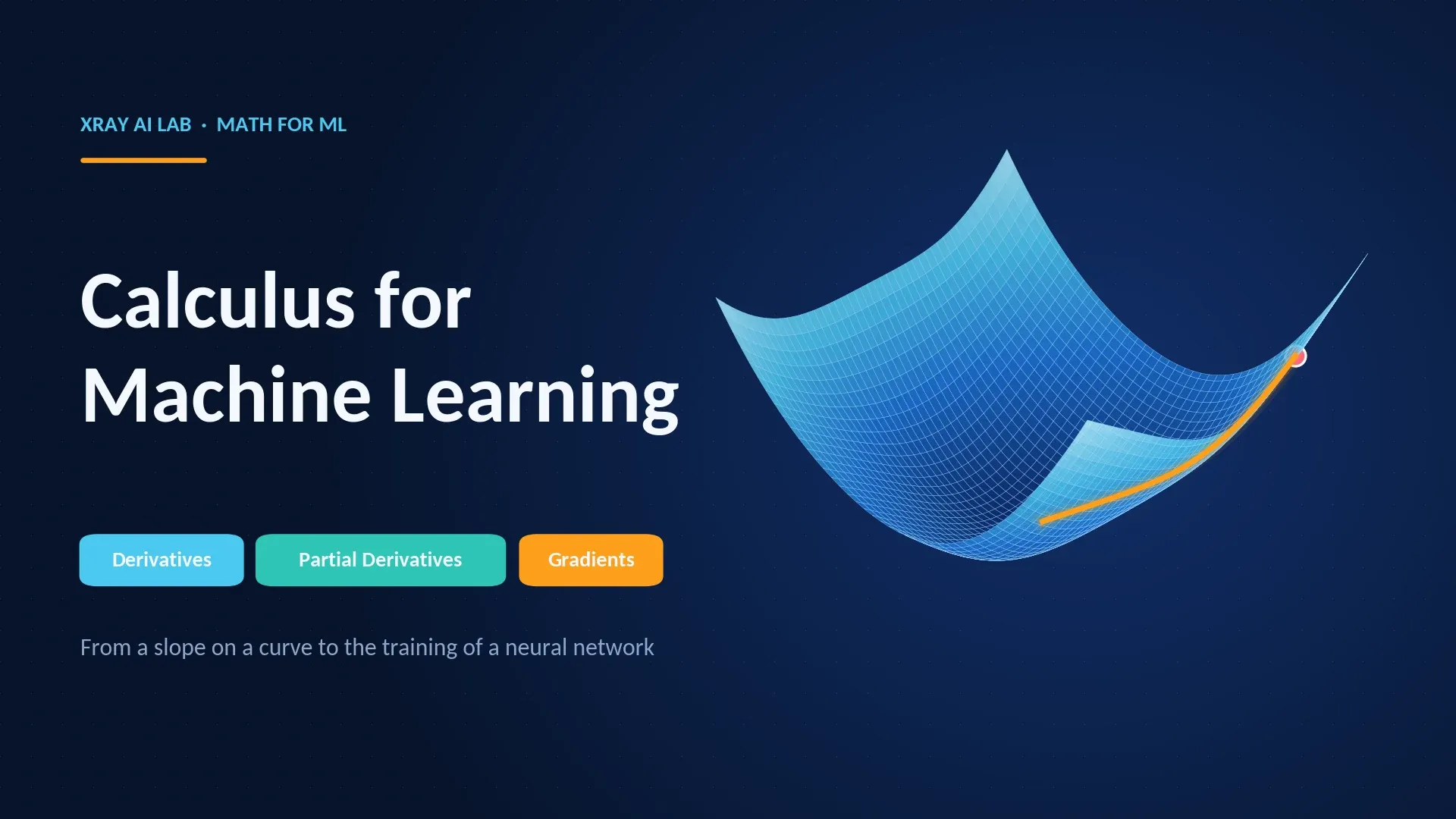
A neural network learns by answering one question over and over: if I nudge this parameter slightly, does the error go up or down, and by how much? Calculus is the tool that answers it. A derivative measures how fast a function changes. A partial derivative does the same when the function has many inputs and you move only one. The gradient collects all the partial derivatives into one vector that points uphill, so training can step the other way.

This guide builds those three ideas in order, starting with pictures. By the end you will be able to:

• explain a derivative as the slope of a tangent line and as a sensitivity,
• compute partial derivatives and assemble a gradient by hand,
• verify your calculus with a numerical gradient check in Python,
• follow how gradients, the chain rule, and the update rule fit together in training.

You only need comfort with algebra and functions. Everything else is introduced as it appears.

Note on the code. Every NumPy and SymPy example in this article was executed (Python 3.12, NumPy 2.4, SymPy 1.14) and the printed output shown is the real output. The PyTorch snippet in the autograd section was reviewed but not executed; its expected output is the analytic result computed in the NumPy example before it.

The Big Picture in One Table

Concept	Question it answers	Role in machine learning
Derivative	How fast does the output change as one input changes?	Sensitivity of the loss to a single parameter
Partial derivative	Same question, when there are several inputs and only one moves	Sensitivity of the loss to one weight among many
Gradient	Which direction increases the output fastest, and how steeply?	The direction gradient descent moves against
Chain rule	How do rates of change combine through stacked functions?	The mathematical core of backpropagation

Part 1: The Derivative, Visually

From secant lines to a tangent line

Take $f(x) = x^2$ and look at the point $x = 3$. The slope of a straight line is easy: rise over run. A curve has a different slope at every point, so we approximate. Draw a secant line through $(3, f(3))$ and a second point a distance $h$ to the right. Its slope is the difference quotient:

$$\frac{f(x+h) - f(x)}{h}$$

Now shrink $h$. The second point slides toward the first, and the secant line rotates until it just grazes the curve. That limiting line is the tangent line, and its slope is the derivative:

$$f'(x) = \lim_{h \to 0} \frac{f(x+h) - f(x)}{h}$$

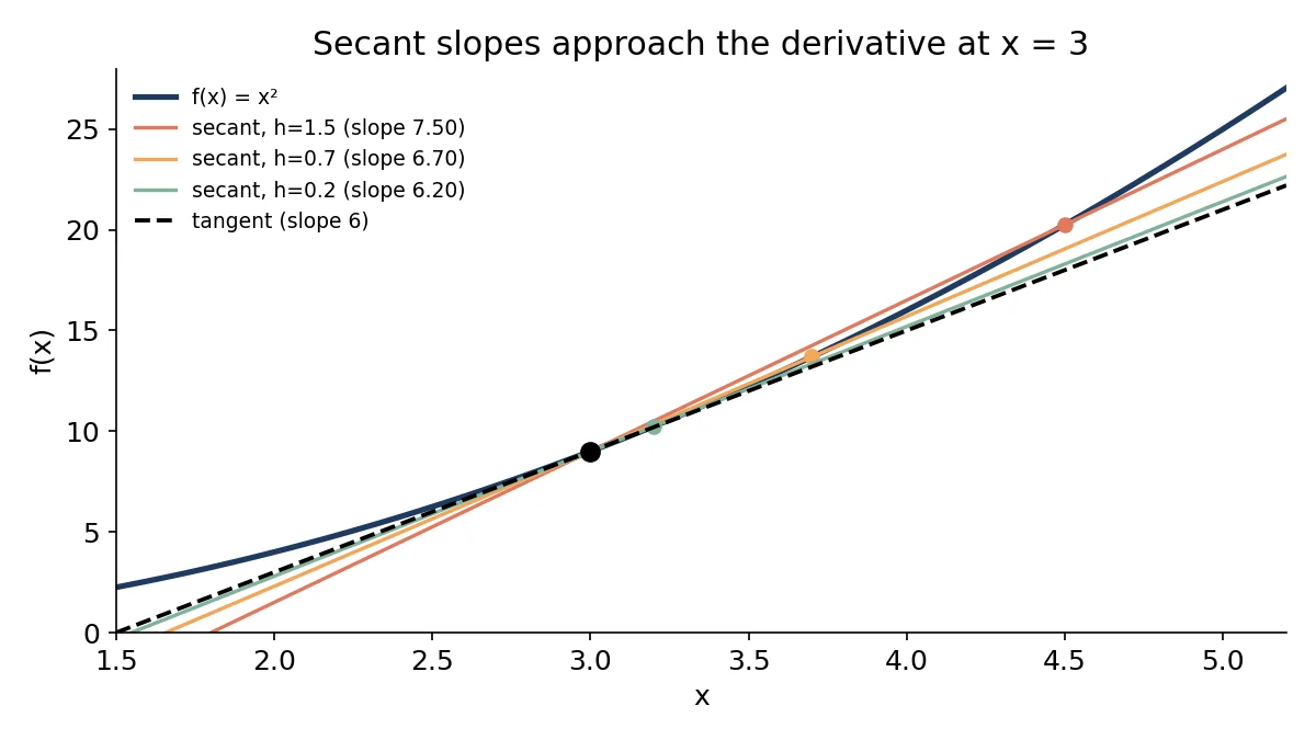
For $f(x) = x^2$ at $x = 3$ we can do the algebra exactly:

$$\frac{(3+h)^2 - 3^2}{h} = \frac{9 + 6h + h^2 - 9}{h} = \frac{6h + h^2}{h} = 6 + h$$

As $h \to 0$ the slope approaches $6$. Python agrees:

def f(x):
    return x**2

x = 3.0
print(f"{'h':>10} {'(f(x+h)-f(x))/h':>18}")
for h in [1, 0.1, 0.01, 0.001, 0.0001]:
    print(f"{h:>10} {(f(x+h)-f(x))/h:>18.6f}")

Output:

         h    (f(x+h)-f(x))/h
         1           7.000000
       0.1           6.100000
      0.01           6.010000
     0.001           6.001000
    0.0001           6.000100

Notice the pattern $6 + h$ in the right-hand column. The derivative is not magic: it is what a very small secant slope settles on.

The derivative as sensitivity

The slope picture has a second, more useful reading for machine learning. Rearranging the definition gives a first-order approximation for small changes $\Delta$:

$$f(x + \Delta) \approx f(x) + f'(x)\,\Delta$$

Read it as: the output changes by about the derivative times the nudge. Suppose a toy loss is $L(w) = (w - 4)^2$ and the current weight is $w = 1$. Then $L'(w) = 2(w-4)$, so $L'(1) = -6$.

• The sign is negative, so increasing $w$ lowers the loss.
• The size says a nudge of $+0.1$ should change the loss by about $-0.6$.

The exact change is $L(1.1) - L(1) = 8.41 - 9 = -0.59$. The approximation is close, and the sign told us which way to move. That is the entire idea behind gradient descent, just in one dimension.

Derivative rules you will actually use

You do not need to take limits every time. A short list covers most of what appears in machine learning:

Rule	Formula
Constant multiple	$(c\,f)' = c\,f'$
Sum	$(f + g)' = f' + g'$
Power	$(x^n)' = n x^{n-1}$
Product	$(fg)' = f'g + fg'$
Chain	$\dfrac{d}{dx} f(g(x)) = f'(g(x))\,g'(x)$
Exponential and logarithm	$(e^x)' = e^x$, $(\ln x)' = 1/x$
Sigmoid $\sigma(z) = \dfrac{1}{1+e^{-z}}$	$\sigma'(z) = \sigma(z)\,(1 - \sigma(z))$
Hyperbolic tangent	$\tanh'(z) = 1 - \tanh^2(z)$
ReLU $\max(0, z)$	$0$ for $z<0$, $1$ for $z>0$

ReLU is not differentiable at exactly $z = 0$. Deep learning libraries simply pick a convention there (commonly $0$), and in practice this rarely matters.

The chain rule is “rates multiply”

Think of three gears. If gear A turns 2 times for every turn of B, and B turns 3 times for every turn of C, then A turns $2 \times 3 = 6$ times per turn of C. The chain rule is that statement for functions: when $y$ depends on $u$ and $u$ depends on $x$,

$$\frac{dy}{dx} = \frac{dy}{du}\cdot\frac{du}{dx}$$

A neural network is a long chain of such dependencies, which is why this rule matters so much. We will use it in a concrete example shortly.

Part 2: Partial Derivatives

One input at a time

Real models have thousands to billions of parameters, so the loss is a function of many variables. Consider a function of two:

$$f(x, y) = x^2 + 3xy + y^2$$

Imagine its graph as a landscape. A partial derivative asks: if I walk exactly parallel to the $x$-axis, how steep is the ground? You freeze $y$ at a constant, treat it like a number, and differentiate with respect to $x$ only:

$$\frac{\partial f}{\partial x} = 2x + 3y \qquad\qquad \frac{\partial f}{\partial y} = 3x + 2y$$

In the first formula, $3xy$ became $3y \cdot x$, so its derivative in $x$ is $3y$ and the $y^2$ term vanished as a constant. The curly $\partial$ is a visual reminder that other variables are being held fixed.

At the point $(1, 2)$:

$$\frac{\partial f}{\partial x}(1,2) = 2(1) + 3(2) = 8 \qquad \frac{\partial f}{\partial y}(1,2) = 3(1) + 2(2) = 7$$

A quick sanity check using the sensitivity idea: $f(1,2) = 11$, and nudging $x$ by $0.01$ should add roughly $8 \times 0.01 = 0.08$. Directly, $f(1.01, 2) = 11.0801$, a change of $0.0801$.

Verifying with code

Two independent checks are better than one: symbolic differentiation with SymPy, and a numerical central difference, which is more accurate than the one-sided quotient we used earlier because the errors on both sides cancel.

import numpy as np
import sympy as sp

def f(x, y):
    return x**2 + 3*x*y + y**2

def numeric_grad(f, point, h=1e-6):
    point = np.asarray(point, dtype=float)
    grad = np.zeros_like(point)
    for i in range(len(point)):
        step = np.zeros_like(point)
        step[i] = h
        grad[i] = (f(*(point + step)) - f(*(point - step))) / (2 * h)
    return grad

x, y = sp.symbols("x y")
expr = x**2 + 3*x*y + y**2
grad_sym = [sp.diff(expr, v) for v in (x, y)]

print("Symbolic gradient:", grad_sym)
print("Symbolic at (1,2):", [g.subs({x: 1, y: 2}) for g in grad_sym])
print("Numeric  at (1,2):", numeric_grad(f, [1, 2]).round(6))

Output:

Symbolic gradient: [2*x + 3*y, 3*x + 2*y]
Symbolic at (1,2): [8, 7]
Numeric  at (1,2): [8. 7.]

The hand calculation, the symbolic result, and the numerical estimate all agree.

Part 3: The Gradient

Collecting partial derivatives into a vector

For a function of $n$ variables, the gradient stacks all $n$ partial derivatives into one vector:

$$\nabla f(\mathbf{x}) = \begin{bmatrix} \dfrac{\partial f}{\partial x_1} \\ \vdots \\ \dfrac{\partial f}{\partial x_n} \end{bmatrix}$$

For our example, $\nabla f(1,2) = [8,\ 7]^\top$. In machine learning the variables are model parameters $\boldsymbol{\theta}$ and the function is the loss $L$, so $\nabla_{\boldsymbol{\theta}} L$ holds one number per parameter, each saying how sensitive the loss is to that parameter.

What the gradient means geometrically

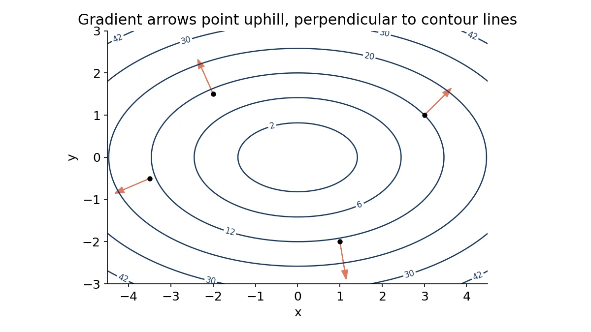
The gradient is more than a bookkeeping device. It has three properties worth memorizing:

1. Direction. It points in the direction of steepest increase of the function.
2. Magnitude. Its length, $\lVert \nabla f \rVert$, is that steepest slope.
3. Orientation. It is perpendicular to the contour lines (the level sets where $f$ is constant).

Why is the gradient the steepest direction? The slope of $f$ along a unit direction $\mathbf{u}$ is the directional derivative

$$D_{\mathbf{u}} f = \nabla f \cdot \mathbf{u} = \lVert \nabla f \rVert \cos\varphi$$

where $\varphi$ is the angle between $\mathbf{u}$ and the gradient. This is largest ($=\lVert\nabla f\rVert$) when $\varphi = 0$, meaning $\mathbf{u}$ points along the gradient, and most negative when $\mathbf{u}$ points directly against it. That is why training moves in the direction $-\nabla L$.

Part 4: How Gradients Train a Model

The gradient descent update

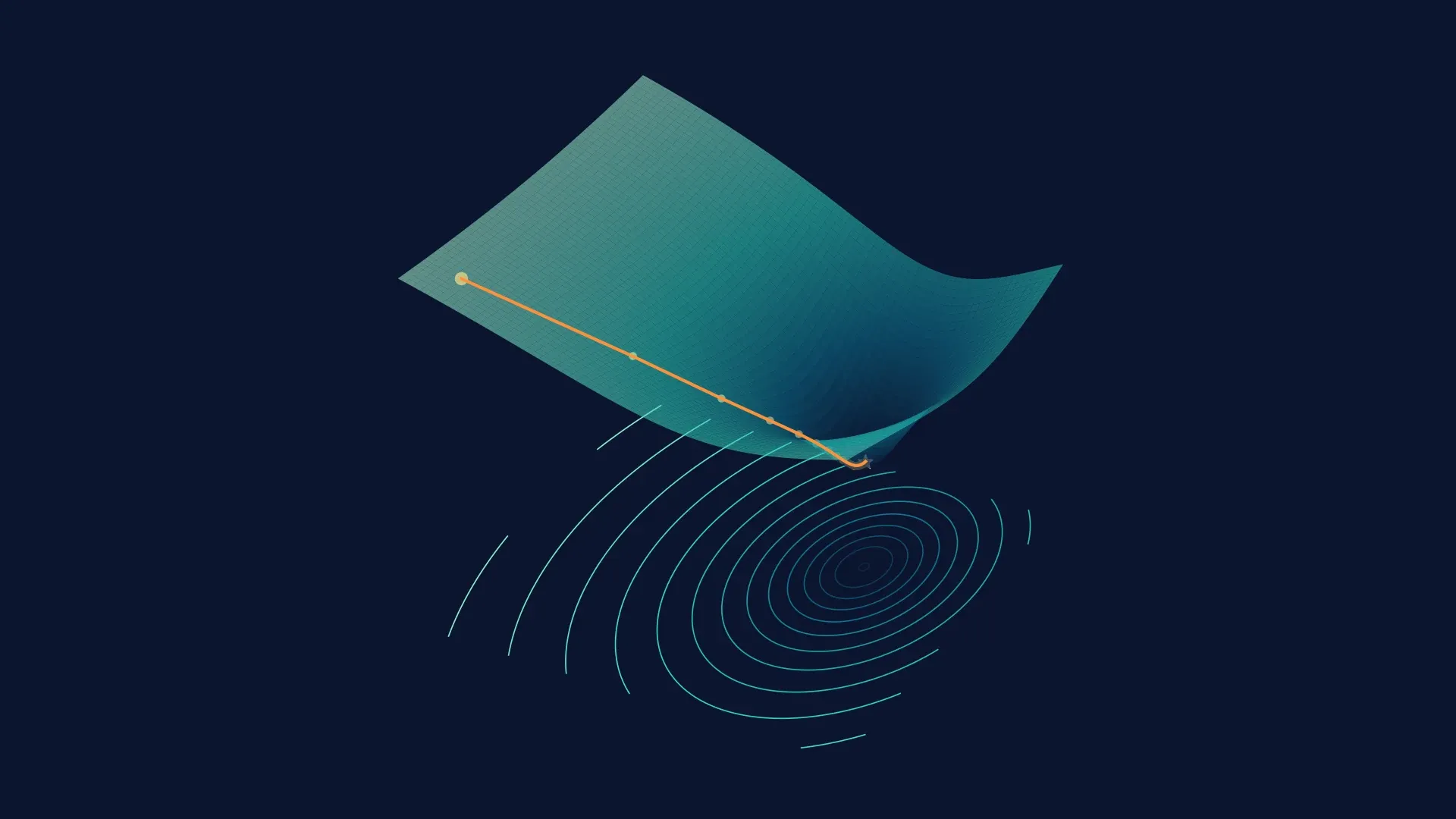
Training turns the geometry above into a loop. Compute the gradient of the loss at the current parameters, then take a small step downhill:

$$\boldsymbol{\theta} \leftarrow \boldsymbol{\theta} - \eta\, \nabla_{\boldsymbol{\theta}} L(\boldsymbol{\theta})$$

The scalar $\eta$ is the learning rate. The minus sign is there because the gradient points uphill and we want to go down.

Here is the loop on a bowl-shaped function $f(x,y) = x^2 + 3y^2$, whose gradient is $\nabla f = [2x,\ 6y]^\top$, starting from $(4, 2)$:

import numpy as np

def grad(p):
    x, y = p
    return np.array([2 * x, 6 * y])

def descend(lr, steps=6, start=(4.0, 2.0)):
    p = np.array(start)
    path = [p.copy()]
    for _ in range(steps):
        p = p - lr * grad(p)
        path.append(p.copy())
    return np.array(path)

for lr in (0.1, 0.4):
    print(f"learning rate = {lr}")
    for k, p in enumerate(descend(lr)):
        print(f"  step {k}: x={p[0]:8.4f}  y={p[1]:9.4f}")

Output:

learning rate = 0.1
  step 0: x=  4.0000  y=   2.0000
  step 1: x=  3.2000  y=   0.8000
  step 2: x=  2.5600  y=   0.3200
  step 3: x=  2.0480  y=   0.1280
  step 4: x=  1.6384  y=   0.0512
  step 5: x=  1.3107  y=   0.0205
  step 6: x=  1.0486  y=   0.0082
learning rate = 0.4
  step 0: x=  4.0000  y=   2.0000
  step 1: x=  0.8000  y=  -2.8000
  step 2: x=  0.1600  y=   3.9200
  step 3: x=  0.0320  y=  -5.4880
  step 4: x=  0.0064  y=   7.6832
  step 5: x=  0.0013  y= -10.7565
  step 6: x=  0.0003  y=  15.0591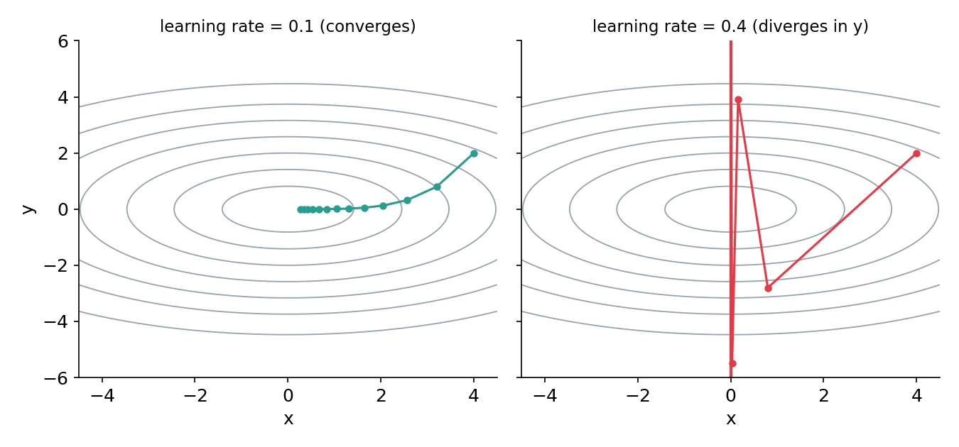

With $\eta = 0.1$ the loss shrinks steadily. With $\eta = 0.4$ it blows up in the $y$ direction even though $x$ is converging. The update rule explains exactly why. Each step multiplies $x$ by $(1 - 2\eta)$ and $y$ by $(1 - 6\eta)$:

• $\eta = 0.1$: factors $0.8$ and $0.4$, both shrink.
• $\eta = 0.4$: factors $0.2$ and $-1.4$. The $y$ coordinate flips sign and grows by 40% each step.

For this function, stability requires $|1 - 6\eta| < 1$, i.e. $\eta < 1/3$. The steepest direction limits how large a learning rate you can use, a small version of what makes real loss surfaces hard to optimize.

Deriving the gradient of a linear regression loss

Now a model with data. Fit $\hat{y} = w x + b$ by minimizing the mean squared error

$$L(w, b) = \frac{1}{n}\sum_{i=1}^{n} \left(w x_i + b - y_i\right)^2$$

Apply the chain rule to each squared term. The outer function is “square” (derivative $2\,\text{error}$) and the inner function is $w x_i + b - y_i$ (derivative $x_i$ with respect to $w$, and $1$ with respect to $b$):

$$\frac{\partial L}{\partial w} = \frac{2}{n}\sum_{i=1}^{n} \left(\hat{y}_i - y_i\right) x_i \qquad\qquad \frac{\partial L}{\partial b} = \frac{2}{n}\sum_{i=1}^{n} \left(\hat{y}_i - y_i\right)$$

Whenever you derive a gradient by hand, check it numerically before trusting it. This is called a gradient check:

import numpy as np

rng = np.random.default_rng(0)
x = rng.uniform(-1, 1, size=100)
y = 2.0 * x + 1.0 + rng.normal(0, 0.1, size=100)   # true w = 2, b = 1, plus noise

def loss(w, b):
    return np.mean((w * x + b - y) ** 2)

def analytic_grad(w, b):
    err = w * x + b - y
    return np.array([2 * np.mean(err * x), 2 * np.mean(err)])

def numeric_grad(w, b, h=1e-6):
    return np.array([
        (loss(w + h, b) - loss(w - h, b)) / (2 * h),
        (loss(w, b + h) - loss(w, b - h)) / (2 * h),
    ])

print("analytic:", analytic_grad(0.0, 0.0))
print("numeric: ", numeric_grad(0.0, 0.0))
print("max abs diff:", np.max(np.abs(analytic_grad(0.0, 0.0) - numeric_grad(0.0, 0.0))))

w, b, lr = 0.0, 0.0, 0.1
for step in range(201):
    gw, gb = analytic_grad(w, b)
    w, b = w - lr * gw, b - lr * gb
    if step % 50 == 0:
        print(f"step {step:3d}  loss={loss(w, b):.4f}  w={w:.3f}  b={b:.3f}")

Output:

analytic: [-1.69404684 -2.3705008 ]
numeric:  [-1.69404685 -2.3705008 ]
max abs diff: 7.216147679400819e-10
step   0  loss=2.1004  w=0.169  b=0.237
step  50  loss=0.0100  w=1.955  b=0.999
step 100  loss=0.0094  w=1.993  b=0.993
step 150  loss=0.0094  w=1.993  b=0.993
step 200  loss=0.0094  w=1.993  b=0.993

The two gradients match to about nine decimal places, so the formulas are right. Training then recovers $w \approx 1.993$ and $b \approx 0.993$, close to the true values $2$ and $1$ but not identical, because the data contain noise. The loss levels off near $0.0094$, which reflects that noise and is not a bug. These numbers apply to this random seed only.

The chain rule through a single neuron

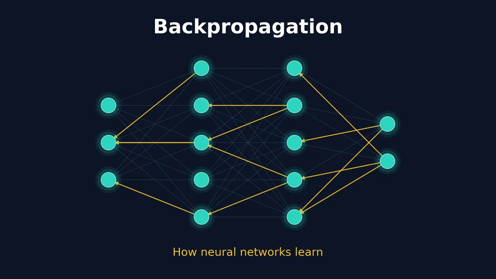
Backpropagation is the chain rule applied systematically through every layer. Its core is visible in a single sigmoid neuron with squared error. Let

$$z = w x + b, \qquad a = \sigma(z), \qquad L = (a - t)^2$$

where $t$ is the target. Chaining the three local derivatives:

$$\frac{\partial L}{\partial w} = \underbrace{2(a - t)}_{\partial L/\partial a}\cdot \underbrace{a(1 - a)}_{\partial a/\partial z}\cdot \underbrace{x}_{\partial z/\partial w}$$

Take $x = 2$, $t = 1$, $w = 0.5$, $b = -1$. Then $z = 0$, so $a = \sigma(0) = 0.5$, and:

• $\partial L/\partial a = 2(0.5 - 1) = -1$
• $\partial a/\partial z = 0.5 \times 0.5 = 0.25$
• $\partial z/\partial w = 2$, $\ \partial z/\partial b = 1$

Therefore $\partial L/\partial w = -1 \times 0.25 \times 2 = -0.5$ and $\partial L/\partial b = -1 \times 0.25 \times 1 = -0.25$. Both are negative, so increasing $w$ or $b$ would reduce the loss. Verified in code:

import math

def sigmoid(z):
    return 1 / (1 + math.exp(-z))

x, t = 2.0, 1.0

def loss(w, b):
    a = sigmoid(w * x + b)
    return (a - t) ** 2

w, b = 0.5, -1.0
a = sigmoid(w * x + b)
dL_da = 2 * (a - t)
da_dz = a * (1 - a)
dL_dw = dL_da * da_dz * x
dL_db = dL_da * da_dz * 1

print("a =", a)
print("dL/dw =", dL_dw, " dL/db =", dL_db)
h = 1e-6
print("numeric dL/dw =", (loss(w + h, b) - loss(w - h, b)) / (2 * h))
print("numeric dL/db =", (loss(w, b + h) - loss(w, b - h)) / (2 * h))

Output:

a = 0.5
dL/dw = -0.5  dL/db = -0.25
numeric dL/dw = -0.5000000000837668
numeric dL/db = -0.2500000000349445

Letting a framework do it: automatic differentiation

Real networks have too many operations to differentiate by hand. Frameworks use automatic differentiation. According to the PyTorch autograd documentation, autograd is a reverse-mode automatic differentiation system that records operations in a graph during the forward pass and then applies the chain rule while traversing it backward. A survey by Baydin, Pearlmutter, Radul, and Siskind (JMLR, 2018) describes backpropagation as a special case of this family of techniques.

Here is the same neuron in PyTorch. This snippet was reviewed but not executed for this article:

import torch

x = torch.tensor(2.0)
t = torch.tensor(1.0)
w = torch.tensor(0.5, requires_grad=True)
b = torch.tensor(-1.0, requires_grad=True)

a = torch.sigmoid(w * x + b)
loss = (a - t) ** 2
loss.backward()

print(w.grad, b.grad)
# Expected from the analytic result above: tensor(-0.5000) tensor(-0.2500)

Two behaviors from the PyTorch documentation matter in training loops. Only leaf tensors with requires_grad=True receive a .grad, and gradients accumulate across backward() calls, so you must reset them between optimizer steps. Optimizers provide zero_grad() for that purpose.

Common Mistakes and Troubleshooting

• Treating the gradient as a scalar. A derivative is a number for one input. A gradient is a vector with one entry per input.
• Wrong sign. Gradient descent subtracts the gradient. Adding it performs gradient ascent and your loss will rise.
• Learning rate too large. If the loss oscillates or explodes, as in the $\eta = 0.4$ run above, reduce $\eta$ before suspecting anything else.
• Differentiating a “held-fixed” variable. In partial derivatives, other variables are constants, not zero. The term $3xy$ contributes $3y$, not nothing.
• Skipping the gradient check. When a hand-derived gradient disagrees with the numerical one by more than roughly $10^{-5}$ in relative terms, the formula (or the code) is usually wrong.
• Choosing $h$ too small in finite differences. Floating-point rounding error grows as $h$ shrinks. Values around $10^{-5}$ to $10^{-6}$ with central differences work well for double precision, and values like $10^{-12}$ do not.
• Forgetting to zero gradients in PyTorch training loops (see above).
• Assuming a zero gradient means a minimum. It could be a maximum or a saddle point. The gradient only describes the surface locally.
• Assuming the minibatch gradient is the true gradient. In practice, training usually estimates the gradient from a small batch, so each step is a noisy approximation.

Practice Exercises

Try each before reading the solution.

1. Find $f'(2)$ for $f(x) = 3x^2 - 2x$.
2. Find both partial derivatives of $f(x, y) = x^2 y + \sin y$ and evaluate them at $(1, 0)$.
3. For $f(x, y) = x^2 + 3y^2$, perform one gradient descent step from $(4, 2)$ with $\eta = 0.1$.

Solutions

1. $f'(x) = 6x - 2$, so $f'(2) = 10$.
2. $\partial f/\partial x = 2xy$ and $\partial f/\partial y = x^2 + \cos y$. At $(1, 0)$: $2(1)(0) = 0$ and $1 + \cos 0 = 2$, so the gradient is $[0,\ 2]^\top$.
3. The gradient at $(4, 2)$ is $[8,\ 12]^\top$. The new point is $(4 - 0.1\cdot 8,\ 2 - 0.1\cdot 12) = (3.2,\ 0.8)$, matching step 1 in the output above.

Frequently Asked Questions

What is the difference between a derivative and a partial derivative?

A derivative applies to a function of one variable. A partial derivative applies to a function of several variables and measures the rate of change along one variable while all the others are held constant.

Why does gradient descent subtract the gradient?

The gradient points toward the steepest increase of the loss. Moving the opposite way decreases the loss fastest locally, which is the direction we want when minimizing.

Is backpropagation the same as the chain rule?

Backpropagation is the chain rule organized efficiently. It computes the gradient of a scalar loss with respect to all parameters by working backward through the network and reusing intermediate results. In the language of automatic differentiation, it is reverse-mode differentiation applied to neural networks.

What is the difference between numerical, symbolic, and automatic differentiation?

Numerical differentiation approximates the derivative with finite differences, which is simple but slow for many parameters and subject to rounding error. Symbolic differentiation manipulates formulas to produce an exact expression, as SymPy does. Automatic differentiation computes exact derivatives (up to floating-point precision) of a program by applying the chain rule to its elementary operations, and is what deep learning frameworks use.

How much calculus do I need for machine learning?

For understanding training, the topics in this article are the core: derivatives, the chain rule, partial derivatives, and gradients. Matrix calculus (Jacobians, and Hessians for second-order methods) is a natural next layer. Integrals appear mainly in probability and statistics.

What happens when the gradient is zero?

You are at a stationary point: a minimum, maximum, or saddle point. Gradient descent makes no further progress there. Which one it is requires second-order information such as the Hessian or additional analysis of the loss surface.

Why do I need to check gradients numerically?

Hand-derived gradients and hand-written backward passes are easy to get subtly wrong, and training can still appear to run with incorrect gradients. A central-difference check on a few parameters is a cheap way to catch those errors.

Conclusion

A derivative is the slope you get when a secant line shrinks to a tangent, and it tells you how sensitive an output is to a small nudge. Partial derivatives extend that idea to many inputs by freezing all but one. The gradient assembles them into the uphill direction, and gradient descent walks the opposite way. The chain rule connects the layers, and automatic differentiation applies it for you.

A good next step is to work through backpropagation on a two-layer network by hand, comparing each gradient against a numerical check as we did here. After that, extend this article’s ideas to vectors and matrices with Jacobians and the Hessian, then explore how optimizers such as momentum and Adam modify the plain update rule.

Sources and Further Reading

• PyTorch documentation, Autograd mechanics.
• Atılım Güneş Baydin, Barak A. Pearlmutter, Alexey Andreyevich Radul, Jeffrey Mark Siskind. Automatic Differentiation in Machine Learning: a Survey. Journal of Machine Learning Research, 18(153):1–43, 2018.
• Marc Peter Deisenroth, A. Aldo Faisal, Cheng Soon Ong. Mathematics for Machine Learning. Cambridge University Press, 2020. A free-to-read reference covering vector calculus and optimization in more depth.